.png)

What Selling in a Crash and Waiting to Buy Back Cost
Selling on a day among the worst in a decade and waiting for the market to recover before buying back is a decision investors make. Across 118 instruments it gave up 3.8 points a year against holding on, and sat out 90% of the ten best days.
Quantlake Time in the Market Study · 127 daily series · data through 31 August 2026 · updated 24 September 2026 · refreshed monthly
Two things to take away. Selling after a crash was not what did most of the damage. Waiting to feel safe before buying back was: returning after one month left the median instrument roughly level with holding on (+0.2 points a year), while waiting for the old high cost 3.8 points a year.
By the time the old high returned, 102% of the recovery from the low had already happened. The investor took the whole fall, missed the rebound, and bought back at about the price where the decline began.
This paper measures a decision investors make in falls: selling, then waiting to buy back.
Morningstar's Mind the Gap 2025 puts a number on the aggregate of it. Over the ten years ended 31 December 2024, the average dollar invested in US open-end funds and ETFs earned 7.0% a year while those funds returned 8.2%, a gap of 1.2 points a year worth about 15% of the funds' total return. The report explains the gap by the timing and magnitude of investors' purchases and sales. This paper measures one path to that result.
The rule is the one investors describe when they explain what happened to them. A day arrives that ranks among the worst in years. They sell. They tell themselves they will buy back when conditions settle or when the market recovers what it lost. This paper tests each promise in the data and prices it.
The trigger. A day whose return ranks among the 10 lowest for that instrument over its own trailing ten years, measured at that day's close, so the decision uses only information available at the close. The position is sold at the next fill. Out of the market, the proceeds earn Treasury bills. The median instrument registered about four such days. The rules below differ only in the re-entry condition.
How a trade is filled. A signal read at the close of day t is executed at the open of day t+1 for an ETF and at the close of day t+1 for a fund or an index, which is how a fund order fills. Costs are 1 basis point a switch as the base case, with 5 and 25 also reported. Taxes are not modelled.
What this paper shows
- The wait is what costs. Selling and returning a month later left the median instrument +0.2 points a year against holding on. Selling and waiting for the old high cost 3.8 points a year. Never returning cost 5.6 points.
- The trade bought a shallower fall at that price. The deepest fall was +11.3 points against holding on, shallower in 88% of instruments. The position was invested on 70% of days.
- Selling in tranches cost a fraction as much. Cutting a fifth on each trigger, down to 40%, gave up 1.3 points a year against 3.8 points for selling the lot. Adding a fifth back on each top-10 up day cut that to 0.6 points.
- The cost rose with volatility, the same gradient Morningstar reports in investor returns. Selling gave up 5.3 points a year in the most volatile third of instruments and 1.2 points in the calmest.
What did each way back in cost?
Every figure in this paper is the median instrument unless it says otherwise. Across the instruments the gap to holding on ran −7.1 pts to +0.5 pts for waiting out the old high. The mean runs close to the median: waiting for the old high cost a median 3.8 points a year and a mean 3.8 points. For the rules that come back on an up day, the mean sits 0.2 to 0.5 points below the median, pulled down by a handful of instruments.
The return column is the middle instrument under each rule, and holding on returned 8.7% a year for its middle instrument. The gap column is each instrument's own gap, then its median, so the two medians belong to different instruments: one month reads 8.2% against 8.7% and a gap of +0.2 points.
One rule came out ahead. Returning after one month left the median instrument +0.2 points a year against holding, ahead in 59% of instruments, with a Sharpe ratio of 0.52 against 0.46 for holding and a deepest fall of −28.9% against −35.9%. No other return rule did.
The rest paid for the wait. A three-month delay cost 1.5 points, six months cost 1.5 points, one year cost 3.4 points, and waiting for the old high cost 3.8 points, the largest figure in the table. Never returning sits outside that comparison: with a trigger this rare, the first extreme day ends the strategy, so the figure prices the trigger date rather than a return decision. For reference, it cost 5.6 points a year.
Every rule cut the deepest fall, because time out of the market during a drawdown reduces exposure to it. Only the one-month wait kept the return that paid for the reduction: its Sharpe ratio is 0.52 against 0.46 for holding; waiting for the old high reads 0.32. The last column, share of days invested, explains most of the table.
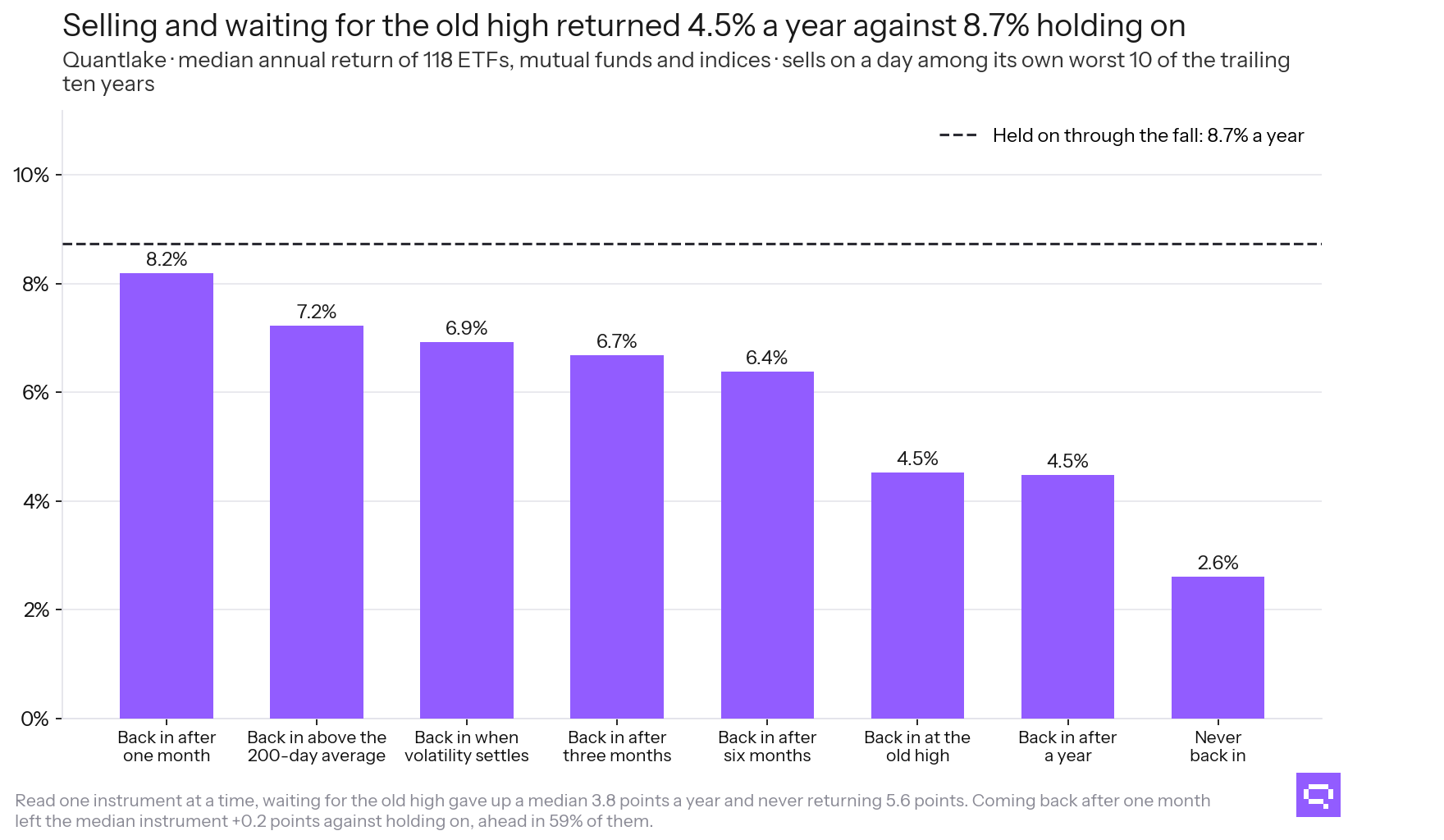
Median annual return against holding on through the fall.
Why does waiting for the recovery cost so much?
By the time the old high is regained, the recovery has already occurred. The rule waits for that point by construction.
Measured as the share of the decline already regained on the buy-back day, where 0 marks the low and 100% the prior high: buying back after a month occurred at 22% of the recovery; waiting for the 200-day average occurred at 34%; waiting for the prior high occurred at 102%, which captures the full recovery and slightly more.
The investor took the full drawdown and bought back at the starting price, earning bill rates in between.
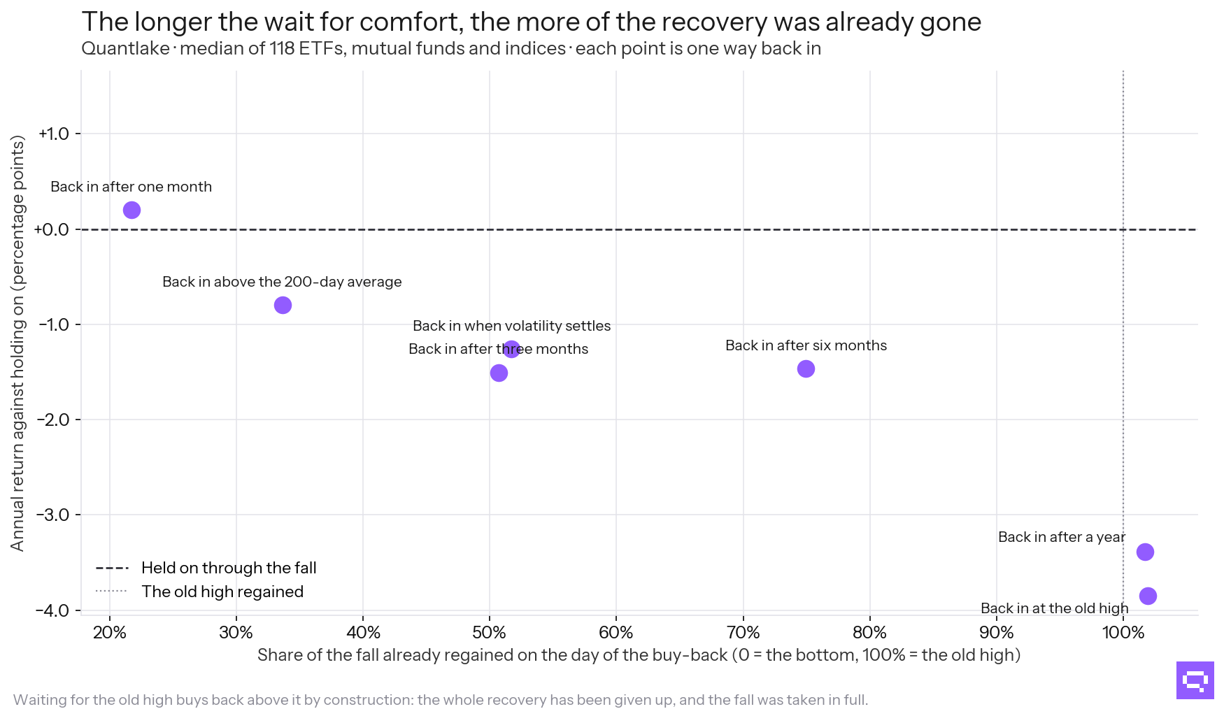
Each point is one way back in, placed by where it bought and what it cost.
Does selling after a bad day at least cut the drawdown?
Yes, and each way back in paid a different price for it. Waiting for the old high made the median deepest fall +11.3 points against holding on, shallower in 88% of instruments, for 3.8 points a year. Never returning made it +16.3 points for 5.6 points a year. Coming back after a month made it +6.2 points, for +0.2 points a year.
Part of that is exposure. A position out of the market on a share of the days falls less with it, whatever the timing: waiting for the old high was invested on 70% of days. Can a Timing Rule Avoid the Worst Days? prints the share of days each of its rules held the asset beside every figure, for the same reason.
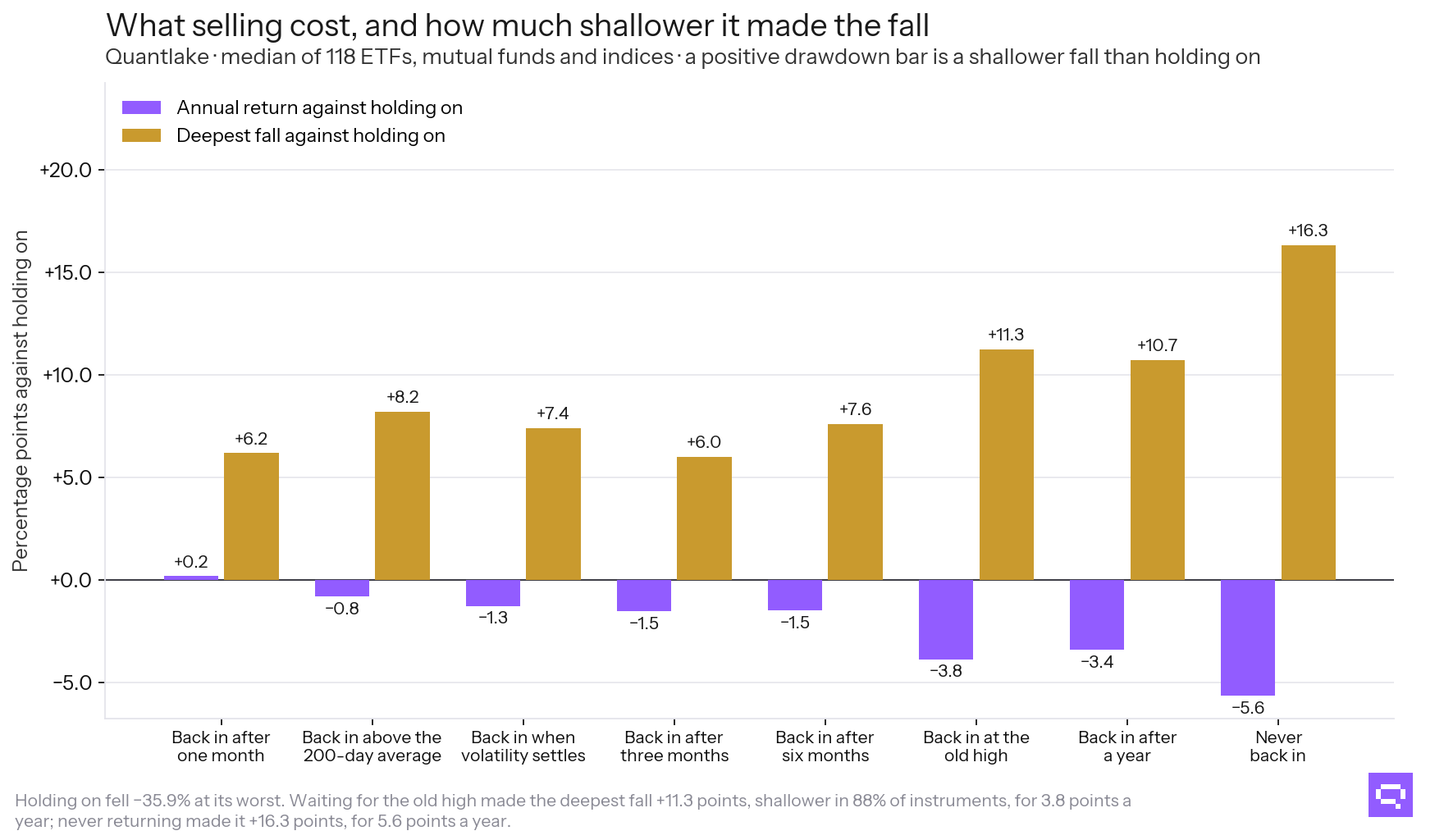
A positive drawdown bar is a shallower fall than holding on.
Does selling in tranches help?
Each trigger cuts a fifth from the holding. The position returns to 100% at the first close that regains the high standing on the day of the first cut. The target does not move as the fall deepens.
Cutting a fifth at a time, down to 40%, a month apart gave up 1.3 points a year against 3.8 points for selling the lot. Its deepest fall was +4.9 points against holding on. Going all the way to zero with no minimum gap between cuts cost 2.9 points, the most of the graded set. A cluster of crash days empties the position inside a week.
The same table shows the graded version out of 26% of the ten best days and 19% of the ten worst, against 90% and 80% for selling the full position.
Every version still trailed holding on.
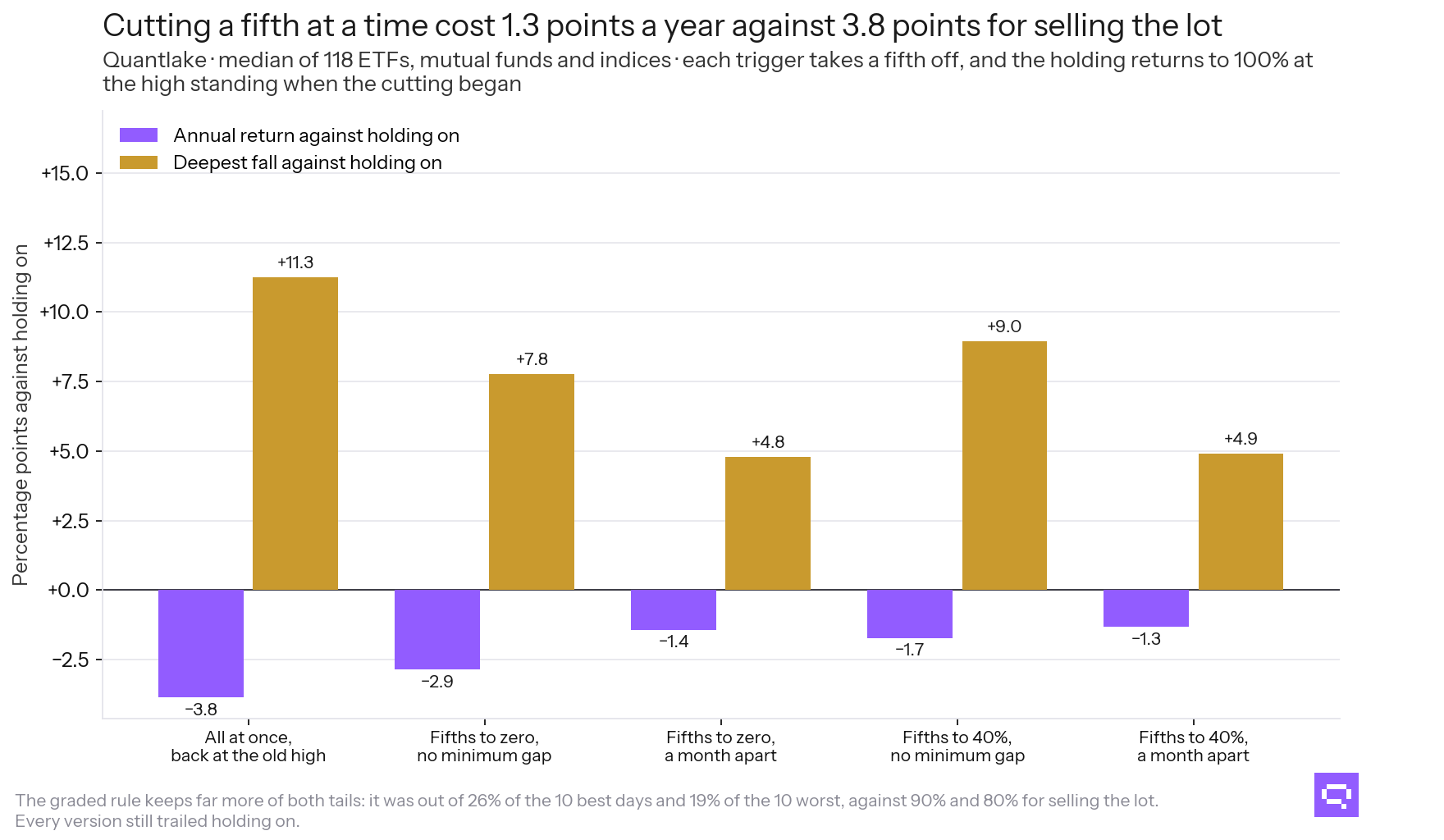
Return and deepest fall, each against holding on through the fall.
Does it depend on how twitchy the trigger is?
Against the trailing ten years, the trigger fires about 4 times. The deepest fall is +11.3 points against holding on, shallower in 88% of instruments, at a cost of 3.8 points a year. Against the trailing five years, it fires about 9 times. The deepest fall is +19.7 points, shallower in 99%, at a cost of 3.8 points a year.
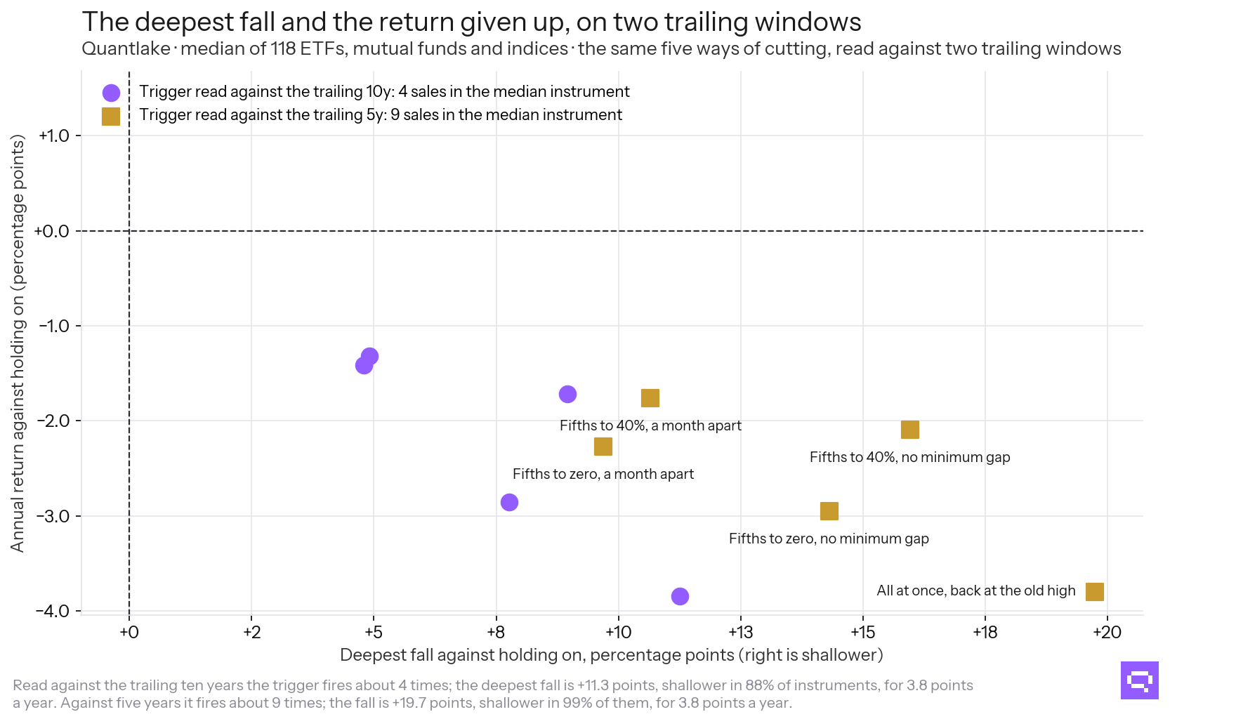
Two trailing windows for the same definition of a crash day.
Does it cost the same whatever you hold?
No. Sorted into thirds by how much they moved over the first year of the window, selling and waiting for the old high cost 5.3 points a year in the third that moved most and 1.2 points in the third that moved least. It beat holding on in 36% of the calmest third and 0% of the stormiest.
On deepest fall, the calmest third was +11.3 points against holding on, shallower in 87% of instruments. The stormiest third was +9.0 points, shallower in 88%.
Mind the Gap 2025 reports the same gradient in real money, measured a different way: the gap between what funds returned and what their investors earned runs 0.4 points a year in the least volatile quintile of funds and 2.0 points in the most (report). In both, the gap widens with volatility.
A rule runs for the whole window, so the group has to be fixed once. These instruments are sorted by the volatility they showed over the first 252 sessions of the scored window, which is the sort an investor choosing between them could have made in advance, and no volatility level decides the boundary. Sorting instead on each instrument's volatility over its whole history, a ranking nobody had at the time, moves the cost to 0.9 points a year in the calmest third and 5.7 points in the stormiest, so the gradient is not what the sort is choosing.
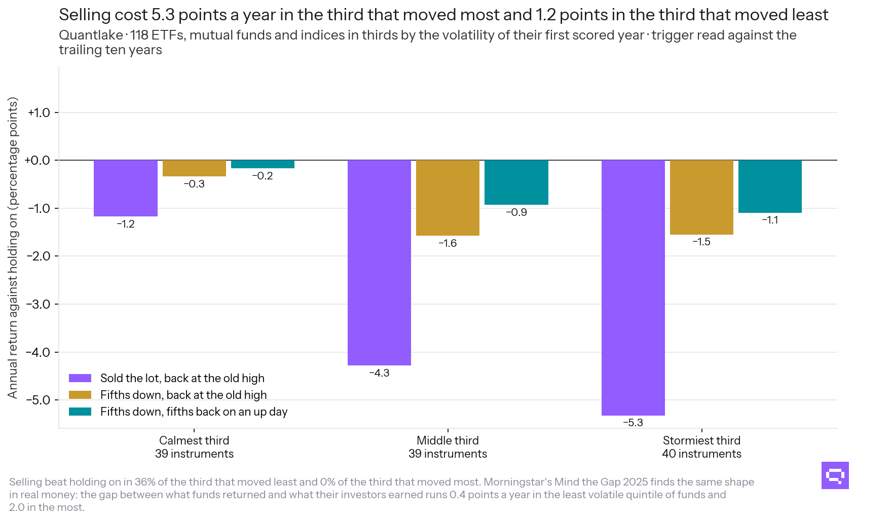
Three ways of cutting, on instruments sorted into thirds by their own volatility.
By asset class, over the ten years, waiting for the old high cost:
| Asset class | Against holding on | Deepest fall | Instruments |
|---|---|---|---|
| Equity | −4.7 pts | +12.3 pts | 76 |
| Credit | −1.2 pts | +11.3 pts | 12 |
| Fixed income | +0.5 pts | +9.3 pts | 18 |
By kind of series, it cost −3.9 points for the median ETF, −1.6 points for the median mutual fund and −4.3 points for the median index series.
The three groups do not cover the same years. The index series run longest and the ETFs shortest, so each lived through a different set of crises, and the funds and indices carry 2000-02, which most ETFs do not. The split checks that the finding holds in each group. It does not rank them.
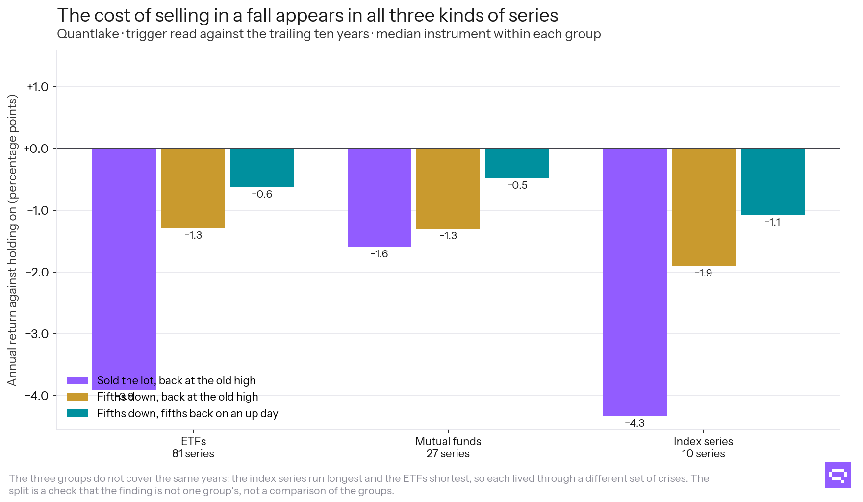
Each group covers a different span of history.
Does it matter whether the day was a fall or a rise?
The trigger so far is a day among the ten worst of the trailing ten years. Its mirror is a day among the ten best, and the same ways back in follow it: an investor who takes money off the table after a spike faces the same question about when to return. The table sets the two triggers side by side.
Selling into strength cost under every return rule, including the one-month rule that paid after a crash. One month out after a top-10 up day left the median instrument −0.7 points a year against holding, where one month out after a top-10 down day left +0.2 points. Waiting for the old high cost 3.7 points against 3.8 points after the down days.
The reason is the clustering again, read from the other side. A top-10 up day sits in the same stretch as the down days, so selling after one puts the investor out through the rest of that stretch, and What Followed the Market's Worst Days measures what came next: a year that returned more than an average one, whichever sign the day carried.
That symmetry is the main result from both papers. Extreme days of either sign mark the same weeks, and a rule that steps out after one steps out through the others.
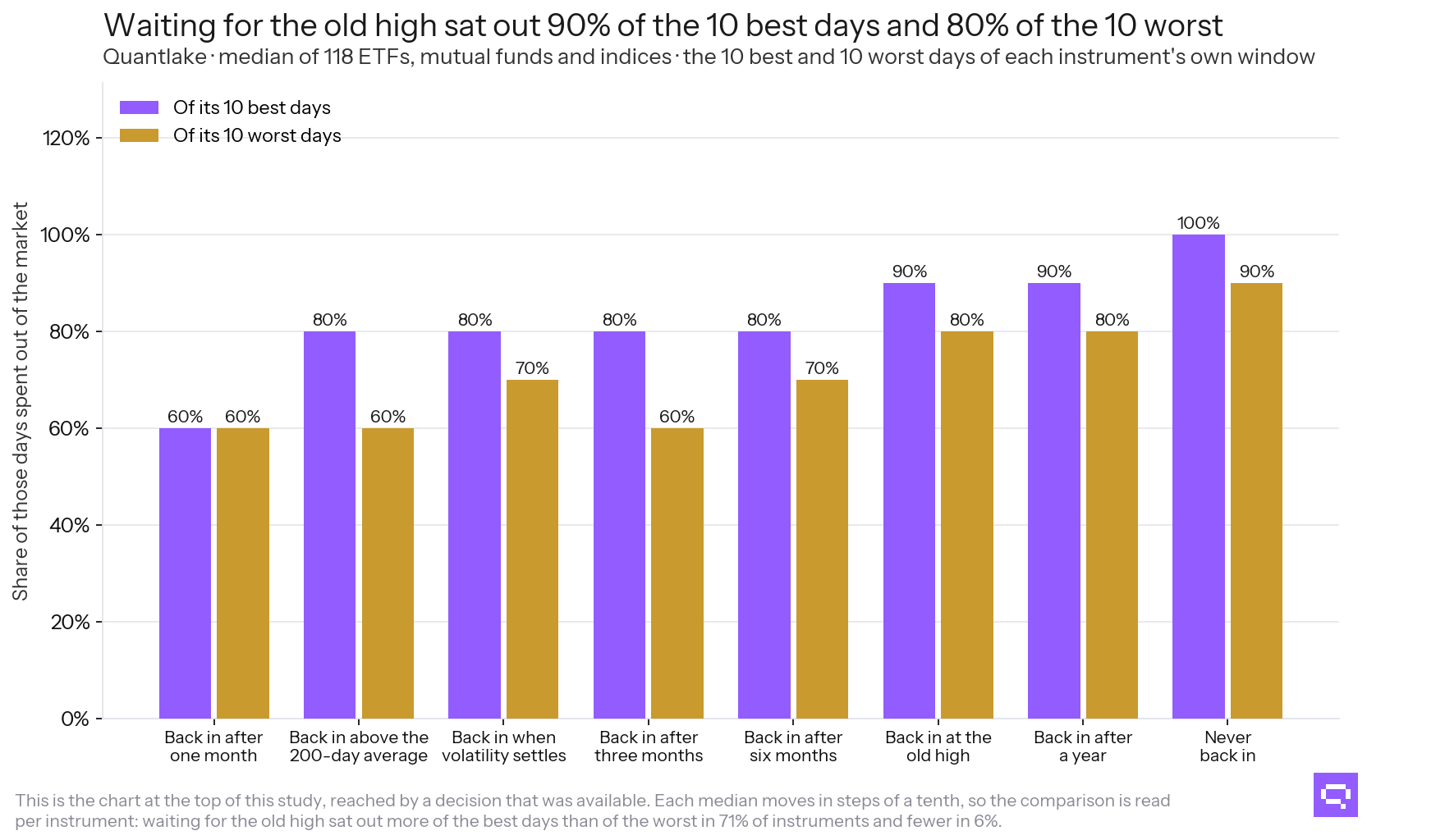
The share of each instrument's 10 best and 10 worst days spent out of the market.
What if a good day is the signal to come back?
It mirrors the trigger. Every rule above picks the way back from the calendar, the price or the volatility. This one reads a top-10 up day of the same trailing window as the signal to return, exactly as a top-10 down day was the signal to leave.
Missing the 10 Best Days predicts the objection: the two kinds of day fall in the same weeks, so a rule that sells on one and buys on the other will trade in and out of the same episode. That is whipsaw. It is measured here as weight traded a year and as the number of times the position left 100% and came back.
Three things come out of that table.
The cooldown made it worse. Switching straight back in on the first top-10 up day cost 1.4 points a year. Making the sale stand for a month first cost 3.4 points. The month-long rule sat out 80% of the ten best days, against 50% for switching straight back.
Grading is the damper that worked. Taking a fifth off on a down day and adding a fifth back on an up day cost 0.6 points a year, against 3.8 points for selling the lot and 1.3 points for cutting in fifths and waiting for the old high. It damps the size of each move and leaves the timing alone. A down day and an up day inside the same week leave the position where it started. It sat out only 28% of the ten best days and 23% of the ten worst.
Costs barely change the result. At a retail 25 basis points a switch, the busiest rule lost a further 0.3 points a year to extra trading, on top of the 1.4 points it gave up at 1 basis point.
Every version still trailed holding on.
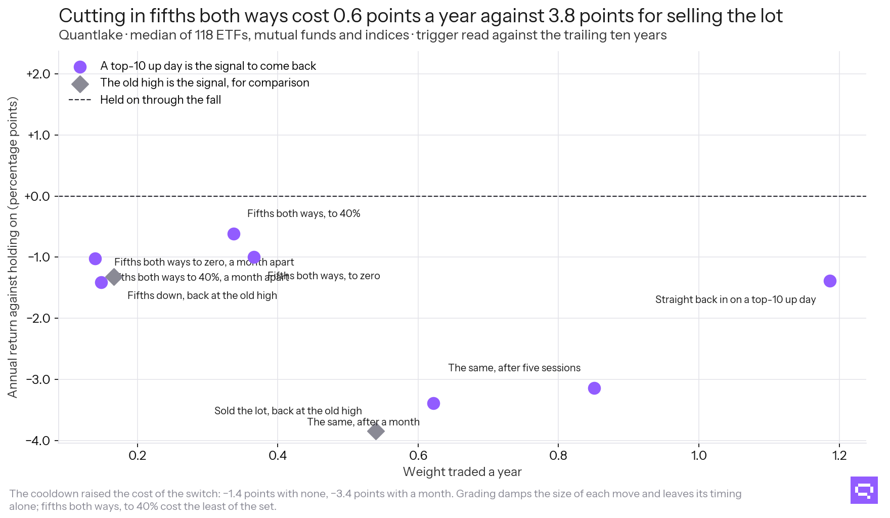
Weight traded a year against the return given up.
How does this connect to the ten-best-days chart?
It reaches the same chart through a decision that was available.
Waiting for the old high sat out 90% of the instrument's ten best days and 80% of its ten worst. Read one instrument at a time, it sat out more of the best than of the worst in 71% of them and fewer in 6%.
33% of these sales were followed within five trading sessions by one of the window's ten best days, the clustering measured in Missing the 10 Best Days.
The ten-best-days chart removes rebounds from the record after the fact. Selling on a crash day and waiting for the old high sat out 90% of the ten best days and cost 3.8 points a year.
What it means
Three things the data supports.
The cost came from the wait. Coming back a month later left the median instrument +0.2 points a year against holding on and ahead in 59% of instruments. Waiting for the old high cost 3.8 points.
Selling made the median deepest fall +11.3 points against holding on when it waited for the old high, and +6.2 points when it came back after a month. The rules tested in Can a Timing Rule Avoid the Worst Days? are measured the same way, against holding the same instrument throughout, with the share of days each rule held it printed beside the figures.
If a position has to be cut in the moment, cutting it in pieces cost a fraction of what cutting it entirely cost here and kept most of the rebound. Letting an equally extreme up day put the pieces back was cheaper still, at 0.6 points a year. Making the rule wait before returning raised the cost.
Which of these numbers applies to a given reader depends on what they hold. For the calmest third of instruments, the whole exercise cost 1.2 points a year and made the deepest fall 11.3 points shallower than holding on. For the stormiest third, the cost was 5.3 points and the deepest fall was 9.0 points shallower. Morningstar reports the same gradient in the money investors actually earned: a gap of 0.4 points a year in the least volatile quintile of funds and 2.0 in the most.
The rules describe a behaviour. They are not candidate strategies, and the measurement is the size of a decision.
Frequently asked questions
Related
- Missing the 10 Best Days: What That Chart Measures
- Can a Timing Rule Avoid the Worst Days? Three Tested
- What Followed the Market's Worst Days, and Its Best
- Does dollar-cost averaging work? A study on ETFs and funds
- Compound interest calculator with volatility, inflation and fees
- Quantlake Time in the Market Study: Method and Data